simple codes on finite element method
Some simple codes on finite element method, including both 1D and 2D case.
有限元模拟的基本步骤包括:
- 建立几何模型
- 网格划分
- 得到有限元矩阵并求解
- 后处理
其中建立几何模型和网格划分往往需要借助CAD,这里介绍的只是对于一些简单的问题如何得到有限元矩阵并求解之。当然,做有限元模拟的大前提是知道物理场的方程是什么以及边界条件是什么。
-
some basic elements
- 网格划分
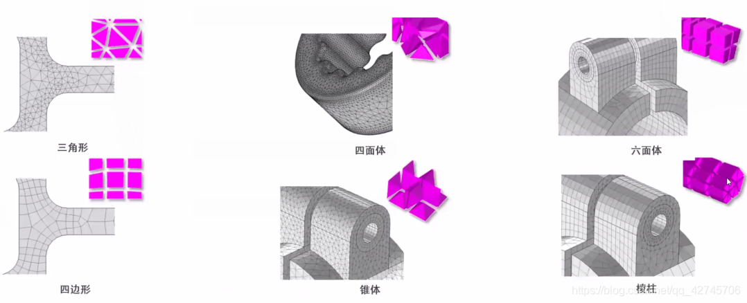
做有限元的第一步通常是网格划分,网格划分有各种类型。
- 形函数
划分完网格之后,要求的就是这些离散格点上的函数值(或者说是物理场的值)。
但是物理场本身是一个连续的量,这就需要用到形函数来构建两者之间的桥梁,将那些非格点的区域的函数形貌用紧邻的格点函数值来描述,当格点越密,这种方式显然是越精确。
一维情形,一阶形函数有两个,
二维情形,在标准单位上的二维形函数有四个,分别为
以及相应的偏导数为 :
习惯上会将它们整合成一个矩阵的形式:
- 雅可比矩阵
在做积分的时候,往往将积分区域通过坐标变换转换为标准区域上的积分,这个变换涉及雅可比矩阵
一维情形的雅可比矩阵为矩阵,;
二维情形的雅可比矩阵为矩阵,,
对于一个任意的四边形(顶角坐标设为),其与标准单位四边形之间的雅可比变换矩阵形式为:
- 速度快且精度高的积分
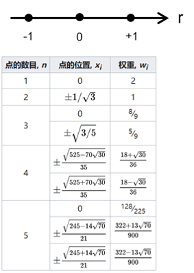
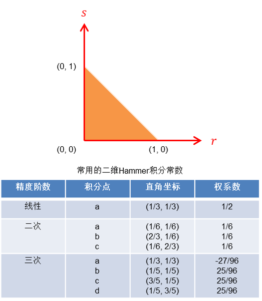
由于通常使用多项式积分,这时候使用高斯求积公式(或Hammer求积公式)会大大提高计算效率,一般情况下用到前几阶的就已经完全严格了。
gauss1
2
3
4
5
6
7
8
9
10
11
12
13
14
15
16
17
18
19
20
21
22
23
24
25%%%%%%%%%%%%%%%%%%%%%%%%%%%%%%%%%%%%%%%%%%%%%%%%%%%%%%%%%%%%%%%%%%%%%%%%%%%
% 根据 order 给出对应的高斯点 gauss_points_list 和 系数 A_coeff_list
%%%%%%%%%%%%%%%%%%%%%%%%%%%%%%%%%%%%%%%%%%%%%%%%%%%%%%%%%%%%%%%%%%%%%%%%%%%
function [gauss_points_list, A_coeff_list] = get_gauss_points(order)
format long % 调整精度
switch order
case 0
gauss_points_list = 0;
A_coeff_list = 2;
case 1
gauss_points_list = [-1/sqrt(3), 1/sqrt(3)];
A_coeff_list = [1, 1];
case 2
gauss_points_list = [-sqrt(0.6), 0, sqrt(0.6)];
A_coeff_list = [5/9, 8/9, 5/9];
case 3
gauss_points_list = [- sqrt(525 + 70 * sqrt(30)) / 35, - sqrt(525 - 70 * sqrt(30)) / 35, sqrt(525 - 70 * sqrt(30)) / 35, sqrt(525 + 70 * sqrt(30)) / 35];
A_coeff_list = [(18 - sqrt(30)) / 36, (18 + sqrt(30)) / 36, (18 + sqrt(30)) / 36, (18 - sqrt(30)) / 36];
case 4
gauss_points_list = [- sqrt(245 + 14 * sqrt(70)) / 21, - sqrt(245 - 14 * sqrt(70)) / 21, 0, sqrt(245 - 14 * sqrt(70)) / 21, sqrt(245 + 14 * sqrt(70)) / 21];
A_coeff_list = [(322 - 13*sqrt(70))/900, (322 + 13*sqrt(70))/900, 0, (322 + 13*sqrt(70))/900, (322 - 13*sqrt(70))/900];
otherwise
error('Gauss Points only available for m = 0,1,2,3,4')
end
endhammer1
2
3
4
5
6
7
8
9
10
11
12
13
14
15
16function [hammer_points_list, A_coeff_list] = get_2d_hammer_points(order)
format long % 调整精度
switch order
case 1
hammer_points_list = [1/3, 1/3];
A_coeff_list = 1/2;
case 2
hammer_points_list = [1/6, 1/6; 2/3, 1/6; 1/6, 2/3];
A_coeff_list = [1/6; 1/6; 1/6];
case 3
hammer_points_list = [1/3, 1/3; 1/5, 1/5; 3/5, 1/5; 1/5, 3/5];
A_coeff_list = [-27/96; 25/96; 25/96; 25/96];
otherwise
error('Hammer Points only available for m = 1, 2, 3')
end
end -
a simple 1D case
It’s very easy to get the answer, so we can use it as a benchmark.
-
单元划分
1
2
3
4
5
6
7
8
9
10
11
12
13
14
15
16
17
18
19
20
21
22
23
24
25
26
27%%%%%%%%%%%%%%%%%%%%%%%%%%%%%%%%%%%%%%%%%%%%%%%%%%%%%%%%%%%%%%%%%%%%%%%%%%%
% test demo in 1D finite element analysis
% (\partial^2 / \partial x^2)u(x) = 2
% with boundary conditions u(1) = u(-1) = 1
%%%%%%%%%%%%%%%%%%%%%%%%%%%%%%%%%%%%%%%%%%%%%%%%%%%%%%%%%%%%%%%%%%%%%%%%%%%
clc;clear
%%%%%%%%%%%%%%%%%%%%%%%%%%%%%%%%%%%%%%%%%%%%%%%%%%%%%%%%%%%%%%%%%%%%%%%%%%%
% 输入参数
%%%%%%%%%%%%%%%%%%%%%%%%%%%%%%%%%%%%%%%%%%%%%%%%%%%%%%%%%%%%%%%%x%%%%%%%%%%%
format long
x_L_end = -1.0;
x_R_end = 1.0;
n_unit = 150;
%%%%%%%%%%%%%%%%%%%%%%%%%%%%%%%%%%%%%%%%%%%%%%%%%%%%%%%%%%%%%%%%%%%%%%%%%%%
% 单元划分
%%%%%%%%%%%%%%%%%%%%%%%%%%%%%%%%%%%%%%%%%%%%%%%%%%%%%%%%%%%%%%%%%%%%%%%%%%%
step_length = (x_R_end - x_L_end) / n_unit;
NE = zeros(n_unit, 2);
node_pos_list = zeros(n_unit + 1, 1); % 每个节点的位置坐标
for i = 1:(n_unit + 1)
if i <= n_unit
NE(i, 1) = i;
NE(i, 2) = i + 1;
end
node_pos_list(i) = x_L_end + step_length * (i - 1);
end -
矩阵组装(体内): $frac{partial^2 u}{partial x^2} = 2$
1
2
3
4
5
6
7
8
9
10
11
12
13
14
15
16
17
18
19
20
21
22
23
24
25
26
27
28
29
30
31
32
33
34
35
36
37
38
39
40order_gauss = 1; % 高斯求积的阶数
[gauss_points_list, A_coeff_list] = get_gauss_points(order_gauss);
%%%%%%%%%%%%%%%%%%%%%%%%%%%%%%%%%%%%%%%%%%%%%%%%%%%%%%%%%%%%%%%%%%%%%%%%%%%
% 矩阵组装 (in the bulk):非边界点
%%%%%%%%%%%%%%%%%%%%%%%%%%%%%%%%%%%%%%%%%%%%%%%%%%%%%%%%%%%%%%%%%%%%%%%%%%%
KG = zeros(n_unit + 1, n_unit + 1);
FG = zeros(n_unit + 1, 1);
KS = zeros(2, 2);
FS = zeros(2, 1);
% 单位元的形函数 ( shape function )
shape_func_matrix = zeros(order_gauss + 1, order_gauss + 1); % 等参变换
shape_func_partial_matrix = zeros(order_gauss + 1, order_gauss + 1);
% 对每个高斯点进行计算
for ii = 1:(order_gauss + 1)
h1 = 1 / 2 * (1 - gauss_points_list(ii)); % h1 = 1 / 2 * (1 - r)
h2 = 1 / 2 * (1 + gauss_points_list(ii)); % h2 = 1 / 2 * (1 + r)
shape_func_matrix(1, ii) = h1;
shape_func_matrix(2, ii) = h2;
shape_func_partial_matrix(1, ii) = - 0.5;
shape_func_partial_matrix(2, ii) = 0.5;
KS = KS - shape_func_partial_matrix(:, ii) * shape_func_partial_matrix(:, ii)';
FS = FS + 2 * shape_func_matrix(:, ii);
end
for ii = 1:n_unit
index_L_end = NE(ii, 1);
index_R_end = NE(ii, 2);
x_L = node_pos_list(index_L_end);
x_R = node_pos_list(index_R_end);
% length of the range
Len_range = (x_R - x_L);
% Jacobi
Jacobi = 1 / 2 * (x_R - x_L);
KG(ii:ii+1, ii:ii+1) = KG(ii:ii+1, ii:ii+1) + KS * Len_range / 2 / (Jacobi)^2;
FG(ii:ii+1) = FG(ii:ii+1) + FS * Len_range / 2;
end -
矩阵组装(边界): $u(1) = u(-1) = 1$
1
2
3
4
5
6
7
8
9
10%%%%%%%%%%%%%%%%%%%%%%%%%%%%%%%%%%%%%%%%%%%%%%%%%%%%%%%%%%%%%%%%%%%%%%%%%%%
% 矩阵组装 (along the edge): 施加边界条件
%%%%%%%%%%%%%%%%%%%%%%%%%%%%%%%%%%%%%%%%%%%%%%%%%%%%%%%%%%%%%%%%%%%%%%%%%%%
KG(1,1) = 1;
KG(1,2:end) = 0;
KG(end,1:end-1) = 0;
KG(end,end) = 1;
FG(1) = 1;
FG(end) = 1; -
求解 + 后处理
1
2
3
4
5
6
7
8
9
10
11
12
13
14
15
16%%%%%%%%%%%%%%%%%%%%%%%%%%%%%%%%%%%%%%%%%%%%%%%%%%%%%%%%%%%%%%%%%%%%%%%%%%%
% 求解函数
%%%%%%%%%%%%%%%%%%%%%%%%%%%%%%%%%%%%%%%%%%%%%%%%%%%%%%%%%%%%%%%%%%%%%%%%%%%
U = KG \ FG;
%%%%%%%%%%%%%%%%%%%%%%%%%%%%%%%%%%%%%%%%%%%%%%%%%%%%%%%%%%%%%%%%%%%%%%%%%%%
% 后处理(作图)
%%%%%%%%%%%%%%%%%%%%%%%%%%%%%%%%%%%%%%%%%%%%%%%%%%%%%%%%%%%%%%%%%%%%%%%%%%%
figure
% 数值解
plot(node_pos_list, U, 'r')
hold on
% 解析解
x_exact = linspace(-1,1,201);
y_exact = x_exact .^ 2;
plot(x_exact, y_exact, 'r--')
-
-
a simple 2D case
-
单元划分
1
2
3
4
5
6
7
8
9
10
11
12
13
14
15
16
17
18
19
20
21
22
23
24
25
26
27
28
29
30
31
32
33
34
35
36
37
38
39
40
41
42
43
44
45
46
47
48
49
50
51
52
53
54
55
56
57
58
59
60
61
62
63
64
65
66
67
68
69
70
71
72
73
74
75
76
77
78
79
80
81
82
83%%%%%%%%%%%%%%%%%%%%%%%%%%%%%%%%%%%%%%%%%%%%%%%%%%%%%%%%%%%%%%%%%%%%%%%%%%%
% test demo in 2D finite element analysis
% 二维泊松方程: \Delta u = 4, -1 <= x,y <= 1
% 边界条件 :
%%%%%%%%%%%%%%%%%%%%%%%%%%%%%%%%%%%%%%%%%%%%%%%%%%%%%%%%%%%%%%%%%%%%%%%%%%%
clc;clear
%%%%%%%%%%%%%%%%%%%%%%%%%%%%%%%%%%%%%%%%%%%%%%%%%%%%%%%%%%%%%%%%%%%%%%%%%%%
% 输入参数
%%%%%%%%%%%%%%%%%%%%%%%%%%%%%%%%%%%%%%%%%%%%%%%%%%%%%%%%%%%%%%%%x%%%%%%%%%%%
format long
X_L = -1.0;
X_R = 1.0;
Y_U = 1.0;
Y_D = -1.0;
np_x = 21;
np_y = 21;
np_node = np_x * np_y;
np_boundary = 2 * (np_x + np_y) - 4;
np_unit = (np_x - 1) * (np_y - 1);
%%%%%%%%%%%%%%%%%%%%%%%%%%%%%%%%%%%%%%%%%%%%%%%%%%%%%%%%%%%%%%%%%%%%%%%%%%%
% 单元划分
%%%%%%%%%%%%%%%%%%%%%%%%%%%%%%%%%%%%%%%%%%%%%%%%%%%%%%%%%%%%%%%%%%%%%%%%%%%
x_value_list = linspace(X_L, X_R, np_x);
y_value_list = linspace(Y_D, Y_U, np_y);
node_pos_list = zeros(np_node, 2);
boundary_list = zeros(np_boundary, 2); % 存放边界点的指标和边界值
unit_index_list = zeros(np_unit, 4); % 每个区域四个点的指标
% 得到 node_pos_list / boundary_list
node_index = 0;
boundary_index = 0;
for j = 1:np_y
for i = 1:np_x
node_index = node_index + 1;
x_value = x_value_list(i);
y_value = y_value_list(j);
node_pos_list(node_index, :) = [x_value, y_value];
% 确定边界节点
if (x_value == X_L) || (x_value == X_R) || (y_value == Y_U) || (y_value == Y_D)
boundary_index = boundary_index + 1;
boundary_list(boundary_index, 1) = node_index;
boundary_list(boundary_index, 2) = x_value^2 + y_value^2;
end
end
end
% 得到 unit_index_list
unit_index = 0;
for j = 1:(np_y - 1)
left_down_index = (j - 1) * np_x;
for i = 1:(np_x - 1)
left_down_index = left_down_index + 1;
unit_index = unit_index + 1;
% left_down
unit_index_list(unit_index, 1) = left_down_index;
% right_down
unit_index_list(unit_index, 2) = left_down_index + 1;
% right_up
unit_index_list(unit_index, 3) = left_down_index + 1 + np_x;
% left_up
unit_index_list(unit_index, 4) = left_down_index + np_x;
end
end
%%%%%%%%%%%%%%%%%%%%%%%%%%%%%%%%%%%%%%%%%%%%%%%%%%%%%%%%%%%%%%%%%%%%%%%%%%%
% 画出网格
%%%%%%%%%%%%%%%%%%%%%%%%%%%%%%%%%%%%%%%%%%%%%%%%%%%%%%%%%%%%%%%%%%%%%%%%%%%
figure
% 撒点
scatter(node_pos_list(:,1),node_pos_list(:,2),'ko','filled');
hold on
% 给每个四边形单元画线
for i=1:np_unit
p = zeros(5,2);
for j=1:4
node_index = unit_index_list(i,j);
p(j,:) = node_pos_list(node_index, :);
end
p(5,:) = node_pos_list(unit_index_list(i,1), :);
plot(p(:,1),p(:,2),'k-');
hold on
end -
矩阵组装(体内)
1
2
3
4
5
6
7
8
9
10
11
12
13
14
15
16
17
18
19
20
21
22
23
24
25
26
27
28
29
30
31
32
33
34
35
36
37
38
39
40
41
42
43
44
45
46
47
48order_gauss = 1; % 高斯求积的阶数
[gauss_points_list, A_coeff_list] = get_gauss_points(order_gauss);
%%%%%%%%%%%%%%%%%%%%%%%%%%%%%%%%%%%%%%%%%%%%%%%%%%%%%%%%%%%%%%%%%%%%%%%%%%%
% 矩阵组装
%%%%%%%%%%%%%%%%%%%%%%%%%%%%%%%%%%%%%%%%%%%%%%%%%%%%%%%%%%%%%%%%%%%%%%%%%%%
KG = zeros(np_node, np_node);
FG = zeros(np_node, 1);
QF = 4; % 微分方程的源,这里取为常数,也可以是x,y的函数
Jacobi_mat = zeros(2, 2);
material_coeff_mat = diag([1,1]); % 可以是介电常数或者其它物理量
[N_mat_list, Nparial_mat_list] = get_jacobi_order1(gauss_points_list); % 计算 N函数 和 N函数偏导 的矩阵
unit_node_pos_list = zeros(4, 2);
% 内部节点
for ii = 1:np_unit
unit_node_indexes = unit_index_list(ii, :);
% 单元上四个节点的坐标
unit_node_pos_list = [node_pos_list(unit_node_indexes(1),:);node_pos_list(unit_node_indexes(2),:); ...
node_pos_list(unit_node_indexes(3),:);node_pos_list(unit_node_indexes(4),:)];
% 得到 KS 和 FS
KS = zeros(4,4);
FS = zeros(4,1);
for jj = 1:2
r_j = gauss_points_list(jj);
A_j = A_coeff_list(jj);
for kk = 1:2
s_k = gauss_points_list(kk);
A_k = A_coeff_list(kk);
Jacobi_mat = Nparial_mat_list(:, :, jj, kk) * unit_node_pos_list; % 该高斯点处的 Jacobi 矩阵
det_Jacobi_mat = abs(det(Jacobi_mat));
J_inv_N_partial_mat = Jacobi_mat \ Nparial_mat_list(:, :, jj, kk);
% 累加 KS 和 FS
KS = KS - A_j * A_k * det_Jacobi_mat * (J_inv_N_partial_mat)' * material_coeff_mat * J_inv_N_partial_mat;
FS = FS + A_j * A_k * det_Jacobi_mat * QF * N_mat_list(:, jj, kk);
end
end
% 将 KS 和 FS 组装进 KG 和 FG 矩阵中
for jj = 1:4
FG(unit_node_indexes(jj)) = FG(unit_node_indexes(jj)) + FS(jj);
for kk = 1:4
KG(unit_node_indexes(jj), unit_node_indexes(kk)) = KG(unit_node_indexes(jj), unit_node_indexes(kk)) + KS(jj, kk);
end
end
end -
矩阵组装(边界)
1
2
3
4
5
6
7
8% 边界节点
for boundary_index = 1:np_boundary
node_index = boundary_list(boundary_index, 1);
node_value = boundary_list(boundary_index, 2);
KG(node_index, :) = 0;
KG(node_index, node_index) = 1;
FG(node_index) = node_value;
end -
求解 + 后处理
1
2
3
4
5
6
7
8
9
10
11
12
13
14
15%%%%%%%%%%%%%%%%%%%%%%%%%%%%%%%%%%%%%%%%%%%%%%%%%%%%%%%%%%%%%%%%%%%%%%%%%%%
% 矩阵求解
%%%%%%%%%%%%%%%%%%%%%%%%%%%%%%%%%%%%%%%%%%%%%%%%%%%%%%%%%%%%%%%%%%%%%%%%%%%
U_numerical = KG \ FG;
U_exact = zeros(np_x, np_y);
for ii = 1:np_x
x_value = x_value_list(ii);
for jj = 1:np_y
y_value = y_value_list(jj);
U_exact(ii, jj) = x_value^2 + y_value^2;
end
end
%%%%%%%%%%%%%%%%%%%%%%%%%%%%%%%%%%%%%%%%%%%%%%%%%%%%%%%%%%%%%%%%%%%%%%%%%%%
% 后处理
%%%%%%%%%%%%%%%%%%%%%%%%%%%%%%%%%%%%%%%%%%%%%%%%%%%%%%%%%%%%%%%%%%%%%%%%%%%
-
simple codes on finite element method
http://example.com/2023/04/26/FEM_simple/


