ABA TLG

Some basic knowledge of ABA tri-layer graphene.

Introduction

Lattice Structure

The lattice structure of ABA tri-layer graphene is shown in the left figure.

It contains six sublattices in its unit cell,

$$A_1, B_1, A_2, B_2, A_3, B_3$$

where A and B refer to the sublattice index while the Arabic number 1,2,3 represent the layer index.

In order to give a precise description of its band structure, the interlayer hopping and intralayer hopping between different sublattice sites need to be considered. Fortunately, it’s enough for most cases to take into account only several of them, which are listed in the table.

hopping direction	$A_n \leftrightarrows B_n$	$B_1 \leftrightarrows A_2 \leftrightarrows B_3$	$A_1 \leftrightarrows A_2 \leftrightarrows A_3$	$A_1 \leftrightarrows B_2 \leftrightarrows A_3$	$A_1 \leftrightarrows A_3$	$B_1 \leftrightarrows B_3$
nominal symbol	$\gamma_0$	$\gamma_1$	$\gamma_4$	$\gamma_3$	$\frac{\gamma_2}{2}$	$\frac{\gamma_5}{2}$

Besides these hopping parameters, the onsite potential also plays an important role in its electronic structure. The onsite potentials on $A_1, B_1, A_2, B_2, A_3, B_3$ are

$$(\Delta_1 + \Delta_2,\quad \Delta_1 + \Delta_2 + \delta,\quad -2\Delta_2 + \delta,\quad-2\Delta_2,\quad-\Delta_1 + \Delta_2,\quad -\Delta_1 + \Delta_2 + \delta )$$

where $\Delta_1$ is the potential difference between the nearest layers which can be controlled by a perpendicular displacement field $\mathbf{D}$ through $\Delta_1 = \alpha d\mathbf{D}$ , where $\alpha$ accounts for the imperfect screening.

$\Delta_2$ is the difference between the potential of the central layer and the averaged potential of outer layers, implying the charge density imblance between the inner and outer layers. It can be expressed as $\Delta_2 = - \frac{4\pi e^2 d}{6\varepsilon_r}n_2$.

and $\delta$ is the dimer site potential.

Therefore, the tight-binding Hamiltonian of ABA TLG in the sublattice basis can be written as

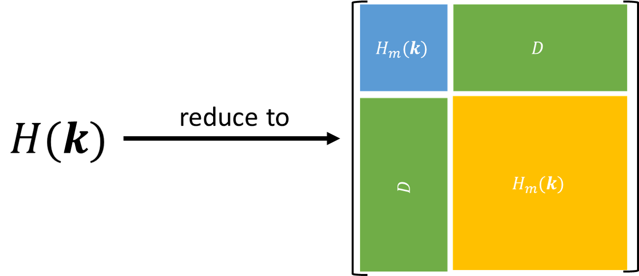
$$\small H(\mathbf{k})=\sum_{\alpha\beta}|\alpha><\alpha|H(\mathbf{k})|\beta><\beta| \\ \tiny =\begin{bmatrix}|A_1> & |B_1> & |A_2> & |B_2> & |A_3> & |B_3>\end{bmatrix} \begin{pmatrix} \Delta_1 + \Delta_2 & \gamma_0 f^{*}(\mathbf{k}) & -\gamma_4 f^{*}(\mathbf{k}) & \gamma_3 f(\mathbf{k}) & \gamma_2 / 2 & 0 \\[6pt] \gamma_0 f(\mathbf{k}) & \Delta_1 + \Delta_2 + \delta &         \gamma_1 & - \gamma_4 f^{*}(\mathbf{k}) &       0 & \gamma_5 / 2\\[6pt]           -\gamma_4 f(\mathbf{k}) & \gamma_1 &   -2\Delta_2 + \delta & \gamma_0 f^{*}(\mathbf{k}) &   -\gamma_4 f(\mathbf{k}) & \gamma_1\\[6pt]     \gamma_3 f^{*}(\mathbf{k}) & -\gamma_4 f(\mathbf{k}) &   \gamma_0 f(\mathbf{k}) & -2\Delta_2 &   \gamma_3 f^{*}(\mathbf{k}) & -\gamma_4 f(\mathbf{k})\\[6pt]     \gamma_2 / 2 & 0 &   -\gamma_4 f^{*}(\mathbf{k}) & \gamma_3 f(\mathbf{k}) &   -\Delta_1 + \Delta_2 & \gamma_0 f^{*}(\mathbf{k})\\[6pt]   0 & \gamma_5 / 2 & \gamma_1 & -\gamma_4 f^{*}(\mathbf{k}) & \gamma_0 f(\mathbf{k}) & -\Delta_1 + \Delta_2 + \delta \end{pmatrix}   \begin{bmatrix}<A_1| \\ <B_1| \\ <A_2| \\ <B_2| \\ <A_3| \\ <B_3|\end{bmatrix}$$

where $f(\mathbf{k})$ is the structure factor associated with the lattice geometry as :

$$f(\mathbf{k}) = e^{-i\mathbf{k\cdot\delta_1}} + e^{-i\mathbf{k\cdot\delta_2}} + e^{-i\mathbf{k\cdot\delta_3}} \approx \left\{ \begin{aligned} -\frac{\sqrt{3}}{2}a(k_x - i k_y) & \quad \text{near } K_{+} \text{ valley}\\ \frac{\sqrt{3}}{2}a(k_x + i k_y) & \quad \text{near } K_{-} \text{ valley} \end{aligned} \right.$$

Mirror Symmetry

Because of its mirror symmetry($|A_1>\longleftrightarrow|A_3>, |B_1>\longleftrightarrow|B_3>$) in the absence of $\mathbf{D}$, the Hamiltonian can be reduced into two blocks, each of which holds a irreducible representation of mirror symmetry, although itself reducible.

First step : basis transformation

$$\tiny \begin{bmatrix} |\phi_1> & |\phi_2> & |\phi_3> & |\phi_4> & |\phi_5> & |\phi_6> \end{bmatrix} = \begin{bmatrix}|A_1> & |B_1> & |A_2> & |B_2> & |A_3> & |B_3>\end{bmatrix} \begin{pmatrix} 1 / \sqrt{2} & 0 & 1 / \sqrt{2} & 0 & 0 & 0 \\[4pt] 0 & 1 / \sqrt{2} & 0 & 1 / \sqrt{2} & 0 & 0\\[4pt] 0 & 0 & 0 & 0 & 1 & 0 \\[4pt] 0 & 0 & 0 & 0 & 0 & 1 \\[4pt] - 1 / \sqrt{2} & 0 & 1 / \sqrt{2} & 0 & 0 & 0 \\[4pt] 0 & - 1 / \sqrt{2} & 0 & 1 / \sqrt{2} & 0 & 0\\ \end{pmatrix}$$

Second step : convert the Hamiltonian into this basis

where

$$H_m(\mathbf{k}) = \begin{pmatrix} -\gamma_2/2 + \Delta_2 & \gamma_0 f^{*}(\mathbf{k}) \\ \gamma_0 f(\mathbf{k}) & \delta - \gamma_5 / 2 + \Delta_2 \\ \end{pmatrix}\\[20pt] H_b(\mathbf{k}) = \begin{pmatrix} \gamma_2/2 + \Delta_2 & \gamma_0 f^{*}(\mathbf{k}) & -\sqrt{2}\gamma_4f^{*}(\mathbf{k}) & \sqrt{2}\gamma_3f(\mathbf{k}) \\ \gamma_0 f(\mathbf{k}) & \delta + \gamma_5 / 2 + \Delta_2 & \sqrt{2}\gamma_1 & -\sqrt{2}\gamma_4f^{*}(\mathbf{k}) \\ -\sqrt{2}\gamma_4f(\mathbf{k}) & \sqrt{2}\gamma_1 & \delta - 2 \Delta_2 & \gamma_0 f^{*}(\mathbf{k}) \\ \sqrt{2}\gamma_3f^{*}\mathbf{k}) & -\sqrt{2}\gamma_4f(\mathbf{k}) & \gamma_0 f(\mathbf{k}) & -2\Delta_2 \end{pmatrix} \\[20pt] D = \begin{pmatrix} \Delta_1 & 0 & 0 & 0 \\ 0 & \Delta_1 & 0 & 0 \end{pmatrix}$$

Continuum Limit

In the continuum limit, the Hamiltonian can be expanded around the two Dirac points $K_{+}$ and $K_{-}$. It makes sense to treat $K_{\pm}$ as a discrete degree of freedom with binary values, called “valley”, which is similar to the spin.

Introduce two operators : $\pi \equiv p_x + i p_y = \hbar (k_x + i k_y), \pi^{\dagger} \equiv p_x - i p_y$

Under a perpendicular magnetic field, $p_x , p_y$ should be replaced by $p_x + eA_x , p_y + eA_y$ (e < 0), then $\pi^{\dagger}/ \pi$ act like creation / annihilation operator, which can be useful in the calculation of Landau level spectra :

$$\pi^{\dagger} \psi_n = i\frac{\hbar}{l_B}\sqrt{2(n+1)}\psi_{n+1} \\ \pi \psi_n = - i\frac{\hbar}{l_B}\sqrt{2n}\psi_{n-1}$$

Introduce other symbols : $v_i = \frac{\sqrt{3}}{2}\frac{a\gamma_i}{\hbar} \text{ for } i = 0, 3, 4$

near $K_{+}$ :

$$H_{m+}= \begin{pmatrix} -\gamma_2 / 2 +　\Delta_2 & -v_0 \pi \\ -v_0 \pi^{\dagger} & \delta - \gamma_5 / 2 + \Delta_2 \end{pmatrix} \longrightarrow \begin{pmatrix} \delta - \gamma_5 / 2 + \Delta_2 & -v_0 \pi^{\dagger} \\ -v_0 \pi & -\gamma_2 / 2 +　\Delta_2 \end{pmatrix} \\$$

exchange the order of basis !!

$$H_{b+}= \begin{pmatrix} \gamma_2 / 2 +　\Delta_2 & -v_0 \pi & \sqrt{2}v_4\pi & -\sqrt{2}v_3\pi^{\dagger}\\ -v_0\pi^{\dagger} & \delta+\gamma_5/2+\Delta_2 & \sqrt{2}\gamma_1 &\sqrt{2}v_4\pi\\ \sqrt{2}v_4\pi^{\dagger} & \sqrt{2}\gamma_1 & \delta - 2\Delta_2 & -v_0\pi \\ -\sqrt{2}v_3\pi & \sqrt{2}v_4\pi^{\dagger} & -v_0\pi^{\dagger} & -2\Delta_2 \end{pmatrix} \\ \longrightarrow \begin{pmatrix} -2\Delta_2 & -\sqrt{2}v_3\pi & \sqrt{2}v_4\pi^{\dagger} & -v_0\pi^{\dagger}\\ -\sqrt{2}v_3\pi^{\dagger} & \gamma_2 / 2 +　\Delta_2 & -v_0 \pi & \sqrt{2}v_4\pi\\ \sqrt{2}v_4\pi&-v_0\pi^{\dagger} & \delta+\gamma_5/2+\Delta_2 & \sqrt{2}\gamma_1\\ -v_0\pi&\sqrt{2}v_4\pi^{\dagger} & \sqrt{2}\gamma_1 & \delta - 2\Delta_2 \end{pmatrix}$$

exchange the order of basis !!

near $K_{-}$ :

$$H_{m-}= \begin{pmatrix} -\gamma_2 / 2 +\Delta_2 & v_0 \pi^{\dagger} \\ v_0 \pi & \delta - \gamma_5 / 2 + \Delta_2 \end{pmatrix}$$

don't need to exchange the order of basis !!

$$H_{b-}= \begin{pmatrix} \gamma_2/2+\Delta_2&v_0\pi^{\dagger}&-\sqrt{2}v_4\pi^{\dagger}&\sqrt{2}v_3\pi\\ v_0\pi & \delta+\gamma_5/2+\Delta_2 & \sqrt{2}\gamma_1 &-\sqrt{2}v_4\pi^{\dagger}\\ -\sqrt{2}v_4\pi & \sqrt{2}\gamma_1 & \delta - 2\Delta_2 & v_0\pi^{\dagger} \\ \sqrt{2}v_3\pi^{\dagger}&-\sqrt{2}v_4\pi&v_0\pi&-2\Delta_2 \end{pmatrix} \\ \longrightarrow \begin{pmatrix} \gamma_2/2+\Delta_2&\sqrt{2}v_3\pi&-\sqrt{2}v_4\pi^{\dagger}&v_0\pi^{\dagger}\\ \sqrt{2}v_3\pi^{\dagger}&-2\Delta_2&v_0\pi&-\sqrt{2}v_4\pi\\ -\sqrt{2}v_4\pi & v_0\pi^{\dagger} & \delta - 2\Delta_2 & \sqrt{2}\gamma_1 \\ v_0\pi &-\sqrt{2}v_4\pi^{\dagger}& \sqrt{2}\gamma_1 &\delta+\gamma_5/2+\Delta_2\\ \end{pmatrix}$$

exchange the order of basis !!

Schrieffer-Wolf Transformation

Although the continuum model describes the low energy regime around charge neutrality point very well, it is still a six-band model. In order to capture the essential of low-energy physics, the $H_{b\pm}$ can be reduced to a $2\times 2$ low-energy effective Hamiltonian :

$$H^{eff}_{b+} = -\frac{1}{2m} \begin{pmatrix} 0 & (\pi^{\dagger})^2 \\ \pi^2 & 0 \end{pmatrix} - \sqrt{2}v_3 \begin{pmatrix} 0 & \pi \\ \pi^{\dagger} & 0 \end{pmatrix} + \begin{pmatrix} -2\Delta_2 & 0 \\ 0 & \gamma_2/2 + \Delta_2 \end{pmatrix} \\[10pt] H^{eff}_{b-} = -\frac{1}{2m} \begin{pmatrix} 0 & (\pi^{\dagger})^2 \\ \pi^2 & 0 \end{pmatrix} + \sqrt{2}v_3 \begin{pmatrix} 0 & \pi \\ \pi^{\dagger} & 0 \end{pmatrix} + \begin{pmatrix} \gamma_2/2 + \Delta_2 & 0 \\ 0 & -2\Delta_2 \end{pmatrix} \\[10pt] \text{where} \quad 1 / 2m = v_0^2 / (\sqrt{2}\gamma_1)[1 + O(\gamma_4 / \gamma_0)^2]$$

Benchmark

The typical values of parameters (in the unit of eV) :

$\gamma_0$	$\gamma_1$	$\gamma_2$	$\gamma_3$	$\gamma_4$	$\gamma_5$	$\delta$	$\Delta_2$	$\alpha$
3.16	0.39	-0.028	0.315	0.12	0.018	0.0355	0.0035	0.3

($\alpha$ describes the imperfect screening effect)

Brief Review of ABA TLG

Here are some papers on ABA TLG

• Band Structure

  1 : Landau level crossing points in ABA TLG at $\mathbf{D=0V/nm}$ can be reflected in the longitudinal magneto-resistance, and they can be used to determine the SWMC parameters.

  2 : $\Delta_2$ is an important parameter in the low-energy physics of ABA TLG

  9 : this theoretical paper tells me that $\Delta_1 = ed\mathbf{D} + \frac{4\pi e^2 d}{2\varepsilon_r}(n_1 - n_3)$(screened by outer layers) and $\Delta_2 = - \frac{4\pi e^2 d}{6\varepsilon_r}n_2$(caused by nonzero charge density on the middle layer), and how to tell whether the disorder strengthen is strong or not (by scanning $\mathbf{D}$ at $\mathbf{B} = 0 T$ to see how sharp the peak at $\mathbf{D} = 0 V/nm$ is).

  3 : hBN substrate can have influence on $\gamma_2, \Delta_2$, the picture is that with substrate, charges from TLG would move towards hBN, which makes the wave functions of the top and bottom layers of TLG shift away from each other and increases the effective distance between them. Therefore, $\gamma_2$ is suppressed while $\Delta_2$ is enhanced.

  4 : ABA TLG at charge neutrality and $\mathbf{D=0V/nm}$ is a semimetal with zero bandgap, but under very high pressure (up to 60GPa), the bandgap can be several eV. To get the gap size, the author uses the following equation

  $$\frac{1}{R(T)} = \frac{1}{R_1(T)}exp[-\frac{E_1}{2k_BT}] + \frac{1}{R_2(T)}exp[-\frac{E_2}{2k_BT}] + \frac{1}{R_3(T)}exp[-(\frac{T_3}{T})^{1/3}]$$

  (the first two terms describe the Arrhenius-like thermally activated conduction process, and the third term describes a Mott variable-range hopping process) to fit the R-T curves.

  5 : This theoretical paper tells me that the screening coefficient $\alpha \approx 0.3$ at not very strong $\mathbf{D}$, through first principle calculation.

  ---

  NOTE

  Q : Why $\Delta_1 = ed\mathbf{D} + \frac{4\pi e^2 d}{2\varepsilon_r}(n_1 - n_3)$ and $\Delta_2 = - \frac{4\pi e^2 d}{6\varepsilon_r}n_2$ ?

  The density on each layer is $n_1, n_2, n_3$. In the absence of $\mathbf{D}$, the mirror symmetry requires $n_1 \equiv n_3$. As a result, the electric field from these two layers cancel each other, so only the electric field from middle layer should be considered. However, in the presence of non-zero $\mathbf{D}$, $n_1$ doesn’t need to be equal with $n_3$, there is a charge imbalance which leads to another net internal electric field $\propto (n_1 - n_3)$.

  ---

• Symmetry Breaking

  6 : This theoretical paper discusses the strong-magnetic-field physics of duodectet subspace of $N = 0$ Landau level in ABC TLG and ABA TLG, using the Hartree-Fock simulation. A Hund’s rules of LL filling order is predicted in ABA TLG.

  7 : At low magnetic field, single particle Quantum Hall picture works well while at higher magnetic field, complete filling of the degeneracy of Lowest Landau Levels (LLL) appears, indicating the physics of quantum hall ferromagnetism. The $\mathbf{D-n}$ measurement at fixed $\mathbf{B}$ also suggests the importance of Coulomb interaction at higher $\mathbf{B}$.

  8 : Quantum Hall Ferromagnetism at finite $\mathbf{B}$, and Fractional QH phases at $\mathbf{D} = 0V/nm$ which disappears at non-zero $\mathbf{D}$.

  10 : Quantum Hall Ferromagnetism at finite $\mathbf{B}$ and hysteresis behavior in longitudinal resistance.

  11 : At low magnetic field $\mathbf{B} = 1.5T$, a symmetry-breaking state at $\nu = 1$ emerges which mainly concentrate in one gully, breaking the $C_3$ symmetry. (penetration field capacitance measurement $C_p = \frac{c^2}{2c + \frac{\partial n}{\partial \mu}}$)

• Edge State

  12 : At low magnetic field $\mathbf{B} \approx 0.5T$, a helical edge state, named “quantum parity hall state” emerges at $\mathbf{D} = 0V/nm$ and $\nu = 0$. The phase diagram at $\nu = 0$ as a function of $\mathbf{D, B_{\perp}, B_{\parallel}}$ is also discussed.

Reference

[1] Quantum Hall effect and Landau-level crossing of Dirac fermions in trilayer graphene | Nature Physics

[2] Phys. Rev. Lett. 117, 066601 (2016) - Landau Level Splittings, Phase Transitions, and Nonuniform Charge Distribution in Trilayer Graphene (aps.org)

[3] Phys. Rev. Lett. 125, 246401 (2020) - Substrate-Dependent Band Structures in Trilayer \mathrm{Graphene}/h\text{\ensuremath{-}}\mathrm{BN} Heterostructures (aps.org)

[4] Large bandgap of pressurized trilayer graphene | PNAS

[5] Phys. Rev. B 92, 245416 (2015) - Density functional theory calculations of the electric-field-induced Dirac cones and quantum valley Hall state in ABA-stacked trilayer graphene (aps.org)

[6] Phys. Rev. B 85, 165139 (2012) - Hund’s rules for the $N=0$ Landau levels of trilayer graphene (aps.org)

[7] Broken Symmetry Quantum Hall States in Dual-Gated ABA Trilayer Graphene | Nano Letters (acs.org)

[8] Phys. Rev. Lett. 117, 076807 (2016) - Tunable Symmetries of Integer and Fractional Quantum Hall Phases in Heterostructures with Multiple Dirac Bands (aps.org)

[9] Phys. Rev. B 79, 125443 (2009) - Gate-induced interlayer asymmetry in ABA-stacked trilayer graphene (aps.org)

[10] Strong electronic interaction and multiple quantum Hall ferromagnetic phases in trilayer graphene | Nature Communications

[11] Phys. Rev. Lett. 121, 167601 (2018) - Emergent Dirac Gullies and Gully-Symmetry-Breaking Quantum Hall States in $ABA$ Trilayer Graphene (aps.org)

[12] Quantum parity Hall effect in Bernal-stacked trilayer graphene | PNAS

Simulation Codes

Band Structure

Band Structure Simulation

No content to show

Landau Level

Landau Level Simulation

No content to show

Hartree Fock Simulation

Above introduce the single-particle simulation of tri-layer ABA graphene, if you are interested in the Hartree Fock simulation of it, please click the link to the page.